Weathering Statics (WXS)
Near surface velocity modeling and correcting for these near surface velocity variations is one of the first steps in seismic data processing. Refraction analysis uses first arrival times of refracted seismic energy to compute near surface velocities and layer thicknesses. Using a combination of proprietary automatic and manual first break picking algorithms we first determine and QC the first break times.
The first break times are used in our WXS interactive/batch software that computes and analyzes weathering models and static corrections. Our method is based on a delay time method of refraction analysis. Within WXS we iteratively compute a weathering model and monitor the fit of the refraction model to the observed data. We interactively QC the model and examine the effect of parameter choices on the resulting model. Figure 1 shows the main window of our interactive statics analysis program. Here we are looking at a single cross-section of a weathering model. In this window we perturb parameters and then examine the effect of changes on the model and the computed statics in map view.
As an example, if the geometry information is correct then the modeled first arrival times should match observed arrival times. A mismatch of the two can represent error in near surface model or placement error of the seismic source and receiver. In Figure 2, such a mismatch is shown, which is in this case due to a shot “skid”. When the shot is moved to the correct position, in Figure 3, the modeled and observed pick times match well.
The velocity depth model from WXS, along with first break time, can be used as input to a subsequent tomographic inversion for near surface velocity depth models.
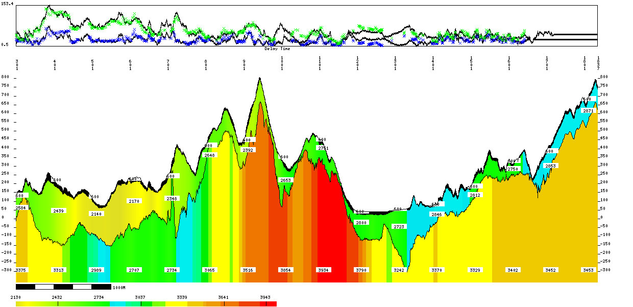
Figure 1. Display of near-surface velocity model cross-section from WXS interactive refractions statics analysis program.
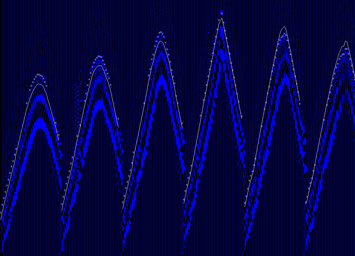
Figure 2. A portion of a shot where the picked times, displayed as "x", do not match the theoretical times shown as a solid yellow line.
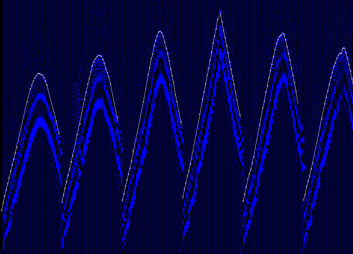
Figure 3. The same data as shown in Figure 2, with a shot skid applied. Now the picked times and modeled time match well.