VVAZ
We perform Velocity Variation with AZimuth (VVAZ) analysis to estimate and correct for azimuthal velocity variations. One cause of azimuthal velocity variations is the presence of horizontal transverse isotropic (HTI) media.
When seismic waves travel through these media the acquired data can exhibit an azimuthal dependence of arrival time. These variations can be observed by constructing a Common Offset Common Azimuth (COCA) display as shown in Figure 1. The sinusoidal variation observed at larger offset on the right of the figure are indicative of azimuthal anisotropy.
An HTI medium is characterized by the azimuth of Vfast, ϕfast, and the percentage of anisotropy, which is a measure of the intensity of the anisotropy and is defined as ((Vfast – Vslow) / Vfast * 100). To calculate these parameters we scan over possible azimuths and percent anisotropy. For each trial value we correct for the azimuthal effect and calculate the semblance in a window around a horizon. Figure 2 shows an example of the semblance from such a scan over a superbin at one CDP location for six horizons. Each of the six windows shows windows semblance as a function of two parameters related to HTI anisotropy. If no azimuthal anisotropy is present the peak of the semblance will occur at the centre of the square. Figure 2 shows that the largest amount of azimuthal anisotropy is present at the fourth horizon, in the lower left corner of the display.
Figure 3 shows the same COCA as in Figure 1, but with and without the VVAZ correction. The correction has, for the most part, removed the azimuthal effect. Figure 4 compares an individual CDP gather with and without the VVAZ correction and shows that the many small trace-to-trace variations observed in the uncorrected gather were due to azimuthal velocity variation.
The deliverables from a VVAZ analysis are corrected gathers and volumes of ϕfast, percent anisotropy, Vfast, and Vslow. The VVAZ corrected gathers are good input to AVO analysis and inversion as the data are better behaved at far angles. The volumes of ϕfast and percent anisotropy can be used to create vector plots as shown in Figure 5 that can be used to identify areas of large anisotropy. The analysis is typically carried out on pre-stack time migrated data, where the migration is run in the common offset vector domain.
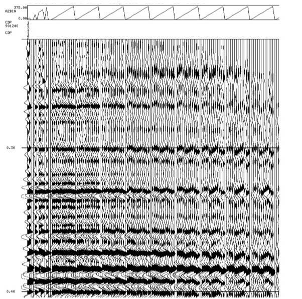
Figure 1. Common Offset Common Azimuth (COCA) display of seismic data.
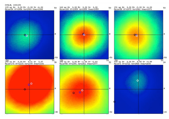
Figure 2. Plot of stack power at six horizons. The x and y axes are related to the degree of azimuthal anisotropy. If the layer is isotropic the semblance peak will be at the centre of the square.
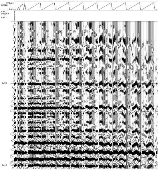

Figure 3. Comparison of a COCA gather with and without VVAZ correction.
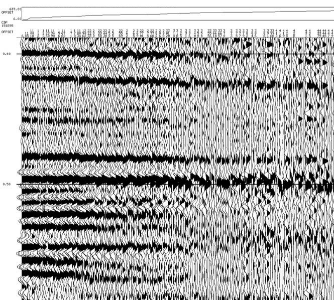
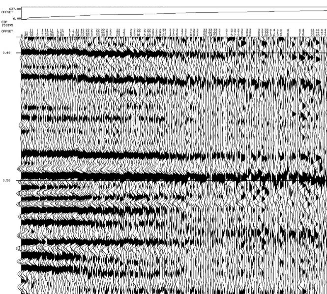
Figure 4. Comparison of a CDP gather with and without VVAZ correction.
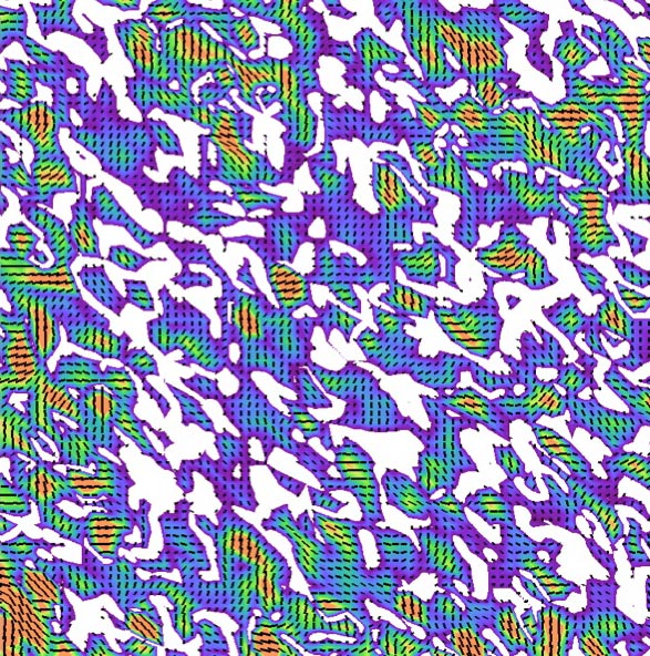
Figure 5. Plot of percent anisotropy for a layer with vectors that point in the azimuth of Vfast and have a length proportional to percent anisotropy.