
SPLITTING ANALYSIS
Historically, shear-wave splitting analysis of PS data has focussed on the detection of fracturing in the subsurface, typically assumed to be represented as a horizontal transverse isotropy (HTI) medium as in Figure 1. An HTI medium is one with a single horizontal axis of symmetry: for example a single set of vertical fractures. As shown in Figure 1 on the left, the converted wave does not undergo splitting in an isotropic medium, however, on the right the shear-wave is split into S1 and S2 modes.
In addition to splitting caused by a fracturing we can also observe shear-wave splitting caused by stress anisotropy. For shallow heavy oil reservoirs the most likely cause of shear-wave splitting is stress anisotropy. There is a great deal of interest in analyzing these stress variations because this analysis may provide valuable input into caprock integrity studies.
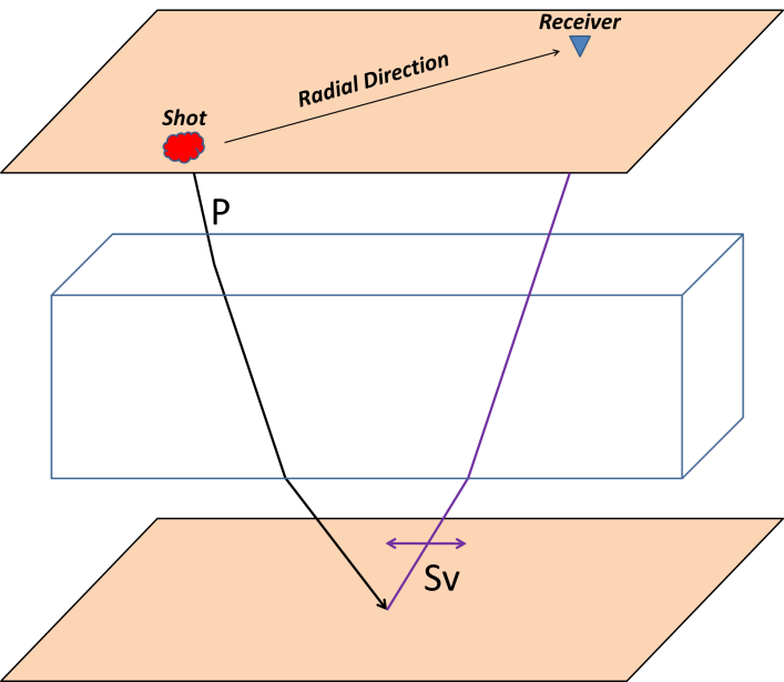
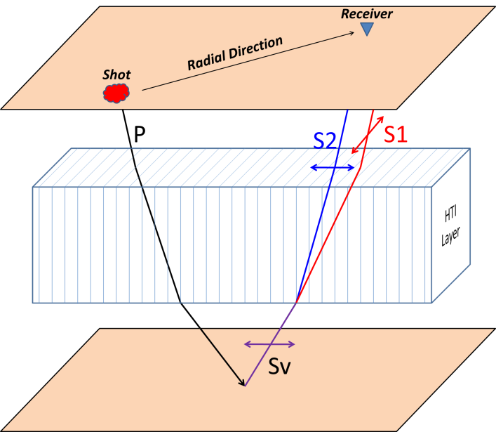
Figure 1. Diagram illustrating the concept of converted-wave splitting in an HTI media. On the left, without HTI anisotropy the wave propagates without splitting . On the right ,with HTI anisotropy the converted wave splits into two modes, labelled S1 and S2. The layering can be thought of as vertical fracturing or regional direction of maximum horizontal stress in the absence of fractures. (From Wikel et al, 2012)
The Shear-wave Splitting Signature
A convenient domain for detection of shear-wave splitting, and analysis of the fast and slow directions or “principal axes”, is after a rotation to radial and transverse directions. Radial refers to the direction aligned with the source receiver azimuth, and transverse is the direction perpendicular to radial. The radial and transverse data can be analysed prestack or after partial stacking into azimuthal sectors. The analysis can also be applied after prestack migration provided that azimuthal information is retained, for example by using a common offset vector (COV) or offset vector tile (OVT) based migration.
In the absence of any azimuthal anisotropy, and assuming a layered medium, there will be no coherent signal present on the transverse component. Therefore, one preliminary indication that shear-wave splitting is present will be observable signal on the transverse component. It should be noted that signal can also arise on the transverse component for other reasons such as structure. The characteristic of splitting related signal is that it will have a 2θ periodicity, with polarity reversals every 90°, and this is generally not the case with other causes of transverse signal. So it is natural to find methods that search for this kind of periodic signal on the transverse data as an indication of probable anisotropy.
To illustrate shear-wave splitting we have constructed a very simple synthetic which consists of a constant medium with 2% difference between S1 and S2 velocities, and a constant S1 azimuth of 30° from north (Figure 2). Four equally spaced reflections have been modelled, and the total amount of time delay between S1 and S2 is simply proportional to reflection time. Thus we can see the progressive change in the nature of the shear-wave splitting signature as the S1-S2 delay time increases. Figure 3 shows a display of the radial and transverse from a dataset acquired over a heavy oil reservoir that displays similar behaviour to the synthetic data.
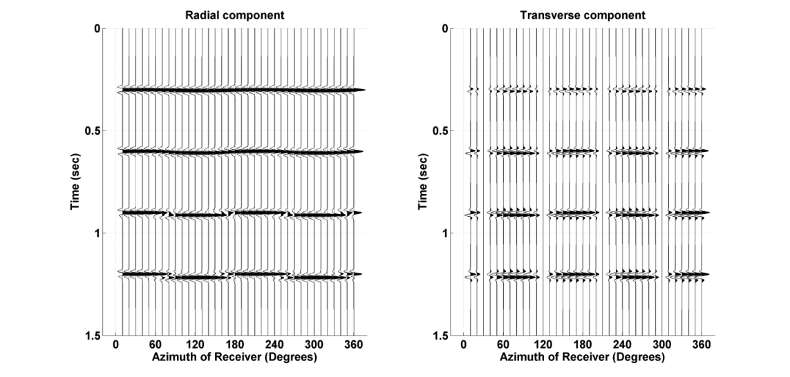
Figure 2. Synthetic gather used to illustrate splitting amplitude effects. Radial component (left) and Transverse component (right) displayed as a function of azimuth from shot to receiver. The S1 direction is 30° and the medium has a constant 2% velocity difference between S1 and S2.
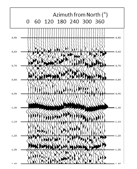
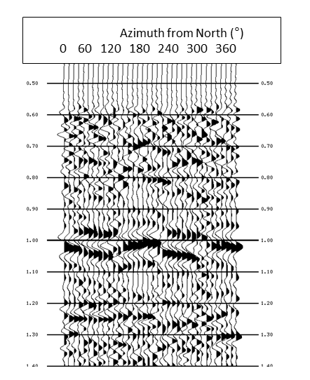
Figure 3. Real data example to illustrate splitting amplitude effects. Radial component (left) and Transverse component (right) displayed as a function of azimuth from shot to receiver. The apparent sinusoidal behaviour of the radial on the left and the polarity flips of the transverse on the right are indicative of shear-wave splitting.
Shear-wave splitting analysis can be viewed as a two-step process: first, estimate orientation of S1 direction, and; second, estimate the time-delay between S1 and S2. Typically we use both Radial and Transverse components to estimate the S1 direction based on amplitude fitting.
Having determined the S1 direction, we next determine the time delay by first applying a rotation to S1 and S2 directions, performing a weighted stack to obtain S1 and S2 traces, and then using a cross-correlation technique. At this point, we have an estimated S1 direction Φ, and time delay Δt, for each CCP location in the survey, at the current analysis depth.
Layer Stripping
Since the earth may contain layers with different stress or fracture regimes, leading to different S1 directions, the recorded shear-waves may have been split multiple times, with both S1 and S2 from the deepest layer being split again into new S1 and S2 directions from the layer above, and so on. This results in considerable complexity of waveform in which the directions for layers are masked by layers above, for all but the shallowest layer. It is important to unravel this effect to find the splitting characteristics at the target depth.
To take into account the existence of several different layers with different S1 directions, we perform layer stripping. In each layer stripping step the estimated time delay is compute as above, then applied on the data after rotation to S1-S2 coordinates, by first shifting the P-S2 data to match P-S1 and then rotating back to the radial-transverse coordinate system. The resulting data may be referred to as radial-prime and transverse-prime (R' and T'). This procedure is illustrated in Figure 4.

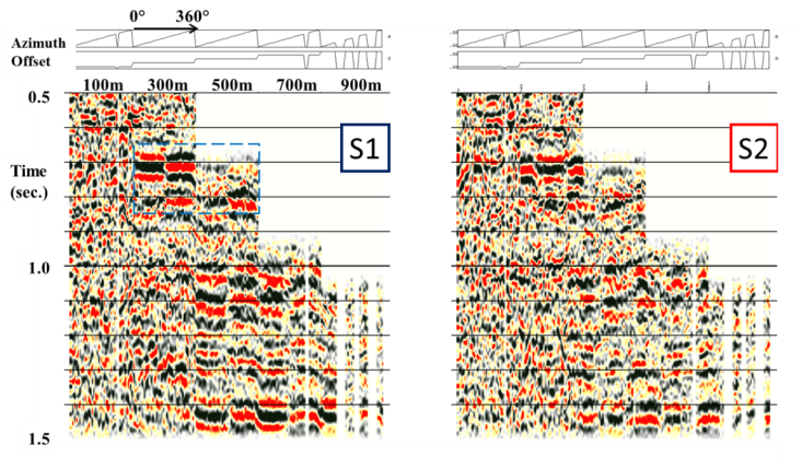
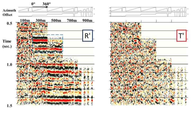
Figure 4. Illustration of transformation from original Radial and Transverse (R-T) coordinates through splitting correction to derive R' and T'. The input common asymptotic conversion point (ACP) gather is at the left, the middle figure shows the gather after rotation to S1 and S2 coordinates and at the right the data displayed after S2 is time shifted and the data are rotated back to R-T. These are now referred to as R' and T'.
At the left the common asymptotic conversion point (ACP) gathers are indexed first by offset range, and then by shot-receiver azimuth, (see profiles above the gathers). The gathers are superbinned using 7x7 bins to improve S/N. Using S1 azimuth derived from the analysis, the data are rotated to the coordinate system defined by S1 and S2 direction. The data in the middle figure are shown after this rotation and with the application of a time delay that is estimated from the analysis (about 10ms) so that the S2 data is shifted upwards to align with the S1 data. Finally in the rightmost figure, the data are rotated back to the R-T coordinate system where the removal of the anisotropy effect is evident. These are referred to as R' and T'.
In order to layer strip through multiple layers, it is necessary to compute R' and T' for each layer in succession, in order to perform analysis for the subsequent layer. Usually the R' dataset is the most suitable for the final goal of imaging the reservoir, although it is also quite possible to generate P-S1 and P-S2 images after the final layer stripping step.
Data Example
An example of the application of shear-wave splitting analysis is shown in Figure 5. In this case, shear-wave splitting analysis over the reservoir interval of an active in-situ combustion project highlights the stress and/or matrix change with time as the combustion front progresses. In this specific case, it is known that the operation is well below the fracture pressure of the interval and that the reservoir itself is not known to be fractured from extensive core samples and logging. The implication of this is that the ample amount of splitting observed in the reservoir (7 ms maximum over a 50 ms layer window), after layer stripping of the above layers, is substantial and most likely due to stress and/or matrix changes within the formation (for more complete information on this example please see Wikel and Kendall, 2012 or Bale et al, 2012).
This type of analysis is useful for gauging the progression of the combustion front along with PP time lapse data and other reservoir engineering information.
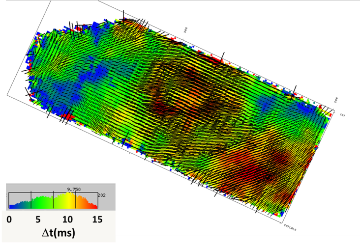
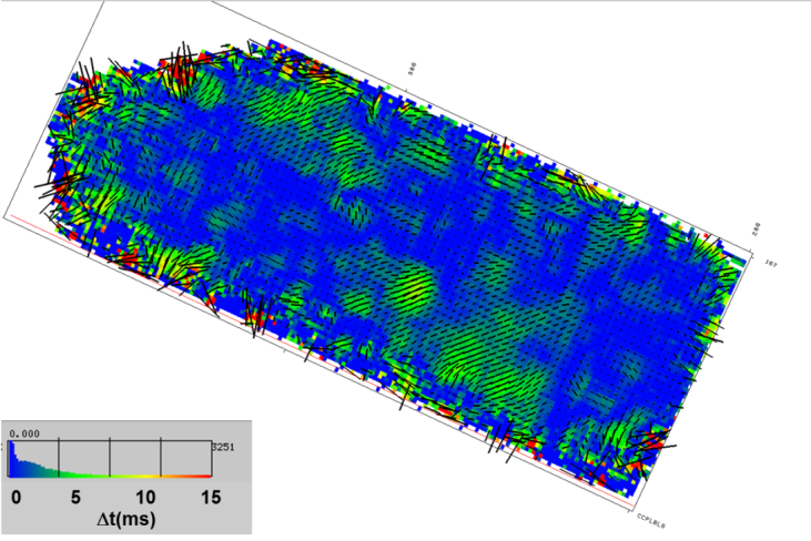
Figure 5. Overburden analysis at left and caprock analysis at right from shear-wave splitting. The colour underlay represents the time delay between S1 and S2 modes, with a range from 0 to 15ms, as shown in the histograms. The line segments represent both time delay (length) and S1 azimuth.