COV
The Common Offset Vector (COV), also known as the Offset Vector Tile (OVT), domain is important in 3D land seismic processing as it provides a natural binning of offsets and azimuths for datasets acquired with a regular acquisition geometry. With an appropriate choice of sampling for the inline and crossline offset, an individual COV is a single-fold dataset with a limited offset and azimuth range. These COVs are an attractive domain in which to apply noise attenuation, FXY interpolation and pre-stack footprint attenuation. Applying pre-stack time migration (PSTM) on COVs allows us to preserve offset and azimuth through migration so that we can perform azimuthal velocity analysis in the migrated location.
A COV is characterized by the sampling of the inline and crossline offset increments. With a regular, orthogonal, 3D acquisition geometry these increments are twice the shot line spacing and twice the receiver line spacing. For merged datasets, or datasets with a great deal of irregularity, we may need to carry out additional analysis to determine the optimal COV parameters. We can perform this analysis interactively and Figure 1 shows the fold of a single COV with inline/xline increments 340/540 m versus 270/540 m. For the nominal acquisition parameters of this survey 340/540 m is the correct choice, but due to variability of the shot and receiver locations 270/540 m is also a good choice. The fold pattern will vary from COV to COV so these must be examined interactively.
This 3D survey is part of a merge and the majority of the data were acquired at a different azimuth and a smaller bin size. (data provided by Strathcona Resources Ltd.) Binning these data with the merge geometry results in the fold, for a single COV, shown in Figure 2.1. After 5D interpolation the fold of the same COV, in Figure 2.2, is now generally single fold for all CDP locations which is ideal for COV PSTM.
When choosing COV processing parameters we can also interactively examine the fold for all COVs for a given inline/xline offset choice as shown in Figure 3. Additionally we can examine the azimuths (Figure 4) and offsets (Figure 5) for the COV geometry. Using these QC plots we can quickly determine the optimal COV parameters for a single 3D survey or a group of surveys in a merge.
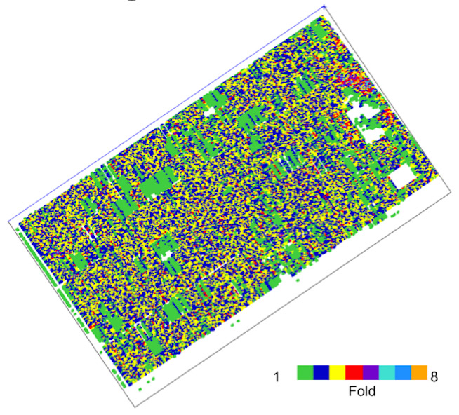
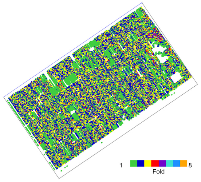
Figure 1. A comparison of fold for an individual COV with inline/xline offset increments of 340/540 m and 270/540 m.
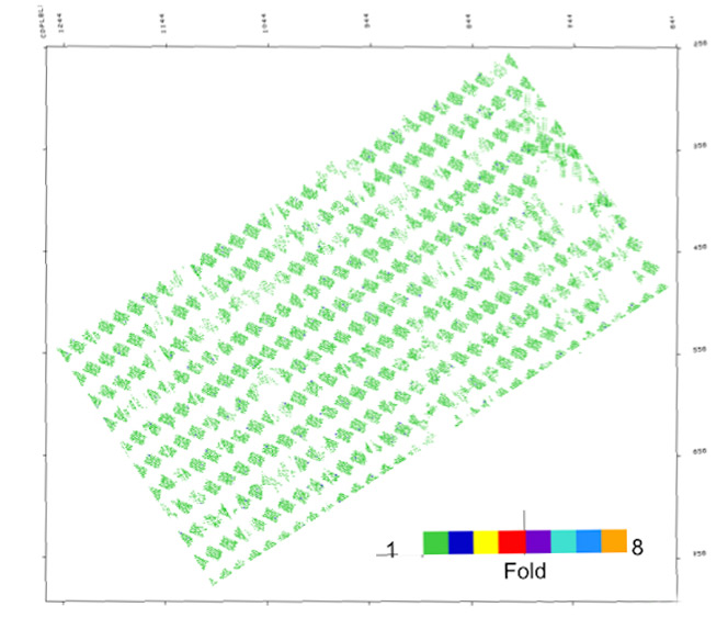
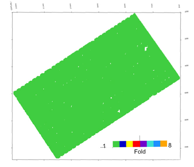
Figure 2. Data from the same survey as shown in Figure 1, however, now in the desired grid for processing of a 3D merge. Shown is fold for a single COV with and without interpolation at the centre of the square.
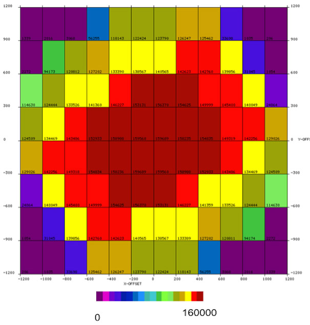
Figure 3. Fold for each COV in a survey as a function X-Offset (inline offset) and Y-Offset (crossline offset). The skewed appearance is a result of the processing grid not being aligned with the acquisition grid.
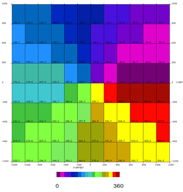
Figure 4. Nominal azimuth for each COV.
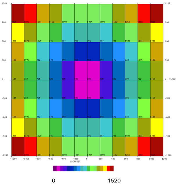
Figure 5. Nominal offset for each COV.